Twitter Sentiment Analysis in R

By Lara Fernandez Musso

The goal of this analysis is to understand the generalized feelings associated with the COVID19 pandemic. To do so, I perform a basic sentiment analysis on Twitter data. I use a dataset collected by Gabriel Preda, which is prepared by running a query for the hashtag #covid19 using the Twitter API alongside Python scripts.

R has an abundance of premade packages that make data analysis infinitely easier. Below, I load in packages that will facilitate data manipulation, processing, and visualization:

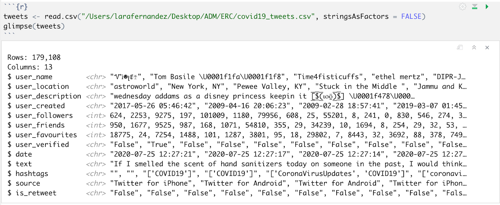
Now, we load in the data. When working with text analysis in R, it is important to set the stringsAsFactors argument of the read.csv function to FALSE, as this ensures that the text is maintained as a string, instead of being converted to a factor variable. The glimpse function allows us to quickly see what our data frame looks like. We have 13 variables (columns) and 179,108 observations/tweets (rows). The variable that is going to be of greatest relevance to us here is “text”, as this is the object that contains the actual tweet itself.

Before getting started with the actual analysis, we need to process, or clean, the data. Text data, especially when coming from internet users, is often very inconsistent. In order for our computer programs to function properly, we need to clean the text for differences that are irrelevant to our analysis. For example, “Covid”, “COVID”, and “covid”, are all the same to us. Differing capitalization does not change what the user is tweeting about.

To standardize our data, we turn to R’s “tm” package. Before performing any operations, we must convert the tweets dataframe to the Corpus format—the data structure used for managing documents in this specific package. 

Now that we have our Corpus, we can perform the following text manipulations:

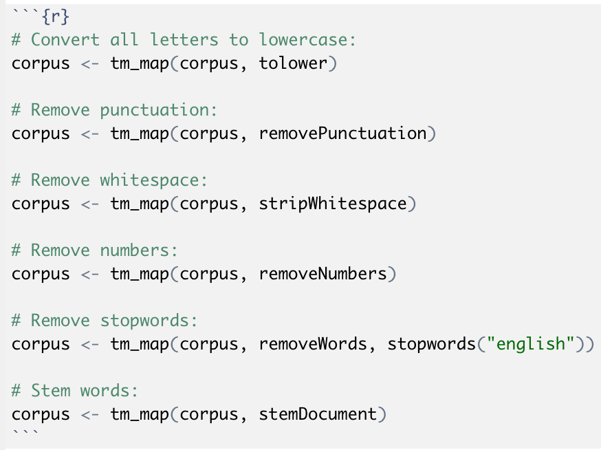
While the first four operations are quite self-explanatory, the last two deserve a brief explanation. Stopwords are words that are commonly used to construct sentences but that don’t really have much meaning by themselves. The following are examples of English stopwords:

To understand stemming, think about the following words: “argue”, “argued”, “argues”, and “arguing”. Although each of these words are used slightly differently in sentences, their core meaning can be represented by the stem “argu”. As with the capitalization example above, there is no reason for our program to differentiate between each of these words, which is why we reduce them all to their stem.

Now that we have cleaned up the text, there is one last necessary pre-processing step: tokenizing the data. In this context, tokenization is the breaking down of human-readable text into algorithm-readable components. Given that our algorithm will analyze sentiment from individual words, it is preferable to have each word in its own separate row in the dataframe. For example, the tweet “COVID is scary” would be tokenized into three separate rows, one containing each word. Note that before tokenizing, we must convert the Corpus object back to a dataframe.

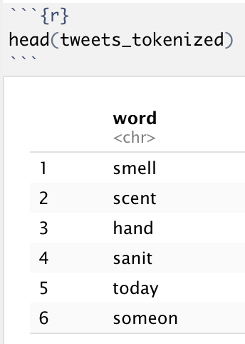
Using the head  or glimpse functions, we can visualize our new dataframe—one column of 2,041,828 rows, where each row is a singular word.

Now that our data has been processed and is ready to go, we can start the analysis. First, I want to see what the most frequently COVID-related words are, as this will provide us with a “big picture” view of what people are thinking regarding the pandemic. We can use the “ggplot2” package to easily visualize the top 10 most frequently occurring word stems.

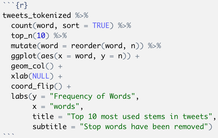
The figure above does not really tell us much about how people are feeling regarding the pandemic. To get a better understanding of this, we can construct a positive-negative sentiment word cloud using lexicons. A lexicon is a dictionary or library that attaches a “sentiment” score to words based on their semantic orientation. These dictionaries are prepared by individuals or built through crowd surfing initiatives. There are three popularly used lexicon libraries in R:

1. Affin: ranks words on a -5 to 5 scare, where -5 is the most negative and 5 is the most positive.
2. Bing: categorizes words in a binary fashion, assigning a value of either positive or negative.
3. NRC: categorizes words as either positive or negative, and then assigns them to one of eight primary emotion categories—anger, fear, anticipation, trust, surprise, sadness, joy, and disgust

Since our word cloud will characterize words as either negative or positive, it makes sense to use the “bing” lexicon. The code below joins the tokenized data frame with the bing library, which we call using the get_sentiments function. The “wordcloud” package then allows us to create the beautiful visualization underneath, which shows us that the most frequently occurring negative words are “death”, “virus”, and “die”, while the most frequently occurring positive words are “trump”, “work”, and “like”. It is curious that “Trump” appears as a positive sentiment…however, we must remember that the lexicon library does not interpret the word “trump” as Donald Trump. The algorithm uses the dictionary definition of “trump”, which is in fact a positive thing: “trump (noun): beat (someone or something) by saying or doing something better”. 

We take this a step further with the “NRC” lexicon, which allows us to count word frequencies by emotion/sentiment category. Surprisingly, the most occurring sentiment is that of trust. I imagine that this is trust towards the medical and scientific community, which is very reassuring! The next most occurring emotions are anticipation, fear, and sadness. This is no surprise, as I can imagine most of us have felt these things over the past year.

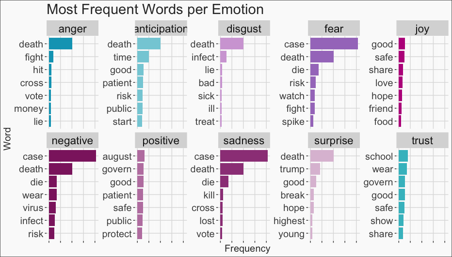
To conclude this analysis, we look within these sentiment categories to see which were the most frequently occurring words in each, once again using the “NRC” lexicon. It’s interesting to see that many words, like “death” or “case”, repeat over multiple sentiment categories.

This type of sentiment text analysis has many useful applications. For example, many businesses use this type of programming to understand how consumers are feeling about their product/brand. I have also seen this being done on the speeches of politicians or on movie scripts. Text analysis is often the first step to a bigger project, like prediction models or recommendation engines.